Integration
Last revision: January 11, 2017Water is flowing from a tap at a rate of $10 \mathrm{l/s}$. After 5 seconds,
how much water has flown? You just multiply: $10 \times 5 = 50 \mathrm{l}$.
But, what if we are told that the flow rate is changing
continuously with time? Let us say that for time
As an approximation, we may split the full time interval into five parts: from $t=0$ to $t=1$, from $t=1$ to $t=2$, etc. For each part, we will assume that the flow rate is constant, and we will choose the value at the beginning. This way, we have:
| Time (s) | Flow rate (l/s) |
|---|---|
| 0 to 1 | 10 |
| 1 to 2 | 5 |
| 2 to 3 | 3.33 |
| 3 to 4 | 2.5 |
| 4 to 5 | 2 |
Now you have to do the product for each part: $10 \times 1 + 5 \times 1 + 3.33 \times 1 + 2.5 \times 1 + 2 \times 1$. Or, the same: $(10+5+3.33+2.5+2) \times 1$. See the idea: we add up the values of the function at the beginning of each part and then multiply by the time interval for each part.
Is this approximation too high or too low? It’s not difficult to see. We have chosen the value at the beginning of the interval, and the function decreases with time, so it must be too high.
What we are trying to compute is the integral of the rate function $r(t)$ from 0 to 5. In mathematical symbols,
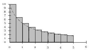
In order to refine the approximation, we should take shorter intervals. For example, half a second. We may try to plot graphically what we’re trying to get. It is really the area under the curve $r(t)$, from $t=0$ to $t=5$. The approximation is the set of rectangles in the following picture:
Can you compute that area with octave? Let us see how. We
should consider all these times: 0, 0.5, 1, 1.5… up to 4.5 (can you
see why?). So, we write
> t=0:0.5:4.5;Now, we want to generate, in a vector, all the values of the function at those times:
> r=10./(t.+1);Now, we sum all those values and multiply by the size of each part, which is 0.5:
> sum(r)*0.5
ans = 20.0199
And get the answer: 20.0199. What would be the exact answer? If you
do the full integration you’ll see that we’re still high…
We can get a lower estimate by using the right extreme of each interval. So, what we do now is
> t=0.5:0.5:5;
> r=10./(t.+1);
> sum(r)*0.5
ans = 16.032
So we know that the right answer lies somewhere in [16.032,20.0199]. We need more precision!!
Can you estimate the value of the integral, giving an upper and a lower bound, using 1000 rectangles?
Making it automatic
Our next challenge will be to write down some octave code that we
can easily use to compute different integrals. We are given the
function $f(x)$, the integration range, $[a,b]$ and the number of
rectangles to use, $N$.
First of all, we compute the width of each rectangle:
> h=(b-a)/N;Now, we find the values of $t$ at the beginning of each rectangle:
> t=a:h:b-h;Why those values? Because the first rectangle starts at $t=a$, the second starts at $t=a+h$… and the last one will start at $t=b-h$. Now we evaluate the function. In the previous case:
> r=10./(1.+t);And now, we sum up:
> sum(r)*hPutting it altogether, we get
> a=0;
> b=5;
> N=100;
> h=(b-a)/N;
> t=a:h:b-h;
> r=10./(1.+t);
> sum(r)*h
ans = 18.128
What if we want to repeat that computation for many values of $N$, in order to see how the result improves? In order to do so we need our first control structure, a for loop.
Let us say that we want to try all $N$ values from 10 to
- Then, we need to do the following:
> a=0;
> b=5;
> for N=10:10:100;
>    h=(b-a)/N;
>    t=a:h:b-h;
>    r=10./(1.+t);
>    sum(r)*h
> endfor
When you do that, you get a lot of numbers, each of one corresponding to a different value of $N$. It would be nicer to put them together, in a vector. Try this other version:
> a=0;
> b=5;
> for N=10:10:100;
>    h=(b-a)/N;
>    t=a:h:b-h;
>    r=10./(1.+t);
>    I(N/10)=sum(r)*h;
> endfor
We have only changed the line in which the value of the sum is
computed. Instead of showing it on the screen, we have stored the
values in a vector I. Try to simply type
> I
I = 20.199 19.010 18.634 18.451 18.342
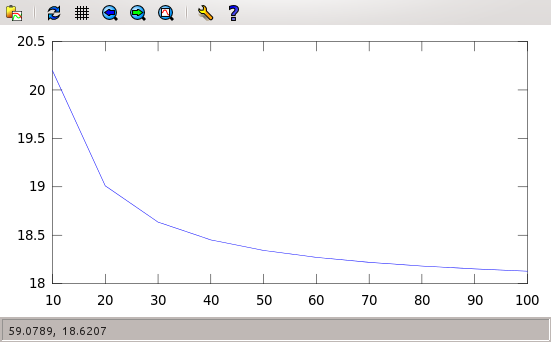
18.270 18.219 18.181 18.152 18.128Why the $N/10$? Because the values of $N$ go as 10, 20, 30… So the components of the vector will be the 1, 2, 3… Now, we can try to plot those values, to see how they approach the right one as $N$ gets large. But, in order to do that precisely, we would like the values of $N$ to get into another vector. That’s easy:
> Nvalues=10:10:100;
> plot(Nvalues,I)
And you should get this:
Trapezoid rule
As you have seen, using the left or the right extreme of each small interval gives a different approximation to the integral. We can do better by using the middle value. This procedure is called the trapezoid rule.
How to do it? Instead of using the left extreme of the
intervals, which is given by a:h:b-a, use the middle
points: a+h/2:h:b-h/2;.
Keep the previous data. Now, we compute a new vector of integral values, doing the following:
> a=0;
> b=5;
> for N=10:10:100;
>    h=(b-a)/N;
>    t=a+h/2:h:b-h/2;
>    r=10./(1.+t);
>    I2(N/10)=sum(r)*h;
> endfor
Now, for the final challenge, we plot them both together:
> plot(Nvalues,I,Nvalues,I2)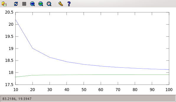
You can see how the errors are much lower in the second case, and the convergence is faster: for lower $N$ we get a more accurate result.
Exercises
-
Estimate the area under a hump of the cosine function.
-
Using the trapezoidal rule, find the area, from $x=0$ to $x=1$, under the curve $y=\sqrt{1-x^2}$. Multiply the result by four. Is this number familiar to you?
-
Get the area under the gaussian $y=\exp(-x^2)$, from $-\infty$ to $\infty$. Find its square. Is this number familiar to you?
-
Use a loop to get the values of the integral, from $x=0$ to $x=1$ of all the functions of the form $f(x)=x^n$, up to $n=10$. Plot the results as a function of $n$. Is the resulting plot familiar to you?