Root finding
Last revision: January 11, 2017Our purpose in this section will be to solve equations numerically, using Newton’s method
Functions in octave
Imagine that you are going to work a lot with a given
function, $f(x)$, and you don’t want to type it continuously. You
can define it for octave in this way:
> function y=f(x)
> y=exp(x)-x;
> endfunction
Now you can call it from the command line, it has become a function
of octave:
> f(1)
ans = 1.7183
The name of the function is f, x is the argument,
and y is the value where you should put the output. Of
course, functions can have any name you want, and they can also take
more than one argument, or can even take vectors as arguments.
Numerical Derivatives
Derivation is a straightforward, but boring task. Imagine that you want to plot a function $f(x)=\sin(\exp(x))$ along with its derivative, $f’(x)$, but you don’t want to take the effort to compute it. Let us do the following: put $f(x)$ in an octave function.
> function y=f(x)
> y=sin(exp(x));
> endfunction
Then, in order to get an approximate value of the derivative around, say, $x=1$, do the following:
> h=0.0001;
> x=1;
> (f(x+h)-f(x))/h
ans = -2.4786
Yes, we know that this formula only returns the derivative when the
limit is taken and $h$ goes to zero. But, still, we can get a
good approximation. In this case, we get -2.4786, while the
real value of the derivative at that point is -2.4783. Fair
enough.
We can use another function:
> function d=df(x)
> h=0.0001;
> d=(f(x+h)-f(x))/h;
> endfunction
This function needs f to be defined in order to work! So, if you
have a well defined f, df is a well defined approximation to the
derivative. Now, in order to plot them, we follow the standard
procedure:
> x1=0:0.001:3.0;
> y1=f(x);
> y2=df(x);
> plot(x1,y1,x1,y2);
Nice, you will see this picture
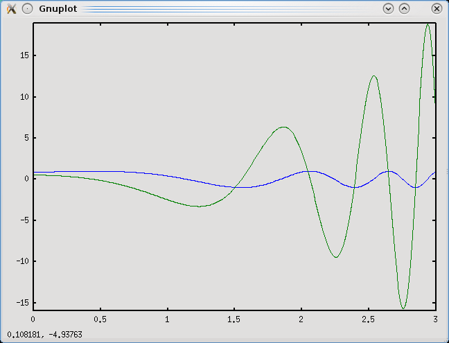
The blue line is the function, the green one the derivative. You can check easily that the maxima and minima of the function coincide with the zeroes of the derivative, as it should.
Script Files
There are functions that you don’t want to type again and again in
octave. So what we can do is to create a script file. This is done
outside. Open any text editor (please, plain text!! No word
documents!!) and type the two functions we have used before, f and
df. Comment lines just should start with # (and it is a good idea
to include comment lines). So, this can be an example:
# Script file that computes a function and its derivative
1; # This is included for technical reasons

# Function f(x) is defined here
function y=f(x)
y=sin(exp(x));
endfunction

# Now, the derivative function df/dx
function d=df(x)
h=0.0001; # Caution! You may want to change this value.
d=(f(x+h)-f(x))/h;
endfunction
This file has to be saved with a name ending in .m. For
example: "functions.m". Now, enter octave and type
> source("functions.m")
> df(1)
And you will get the correct result.
Newton’s method
After a lot of previous work, we come to our original purpose, which is to solve any equation of the type $f(x)=0$ with Newton’s method. Consider the function we have used so far, $f(x)=\sin(\exp(x))$. From the plot, we can roughly see solutions to the equation. For example, there should be a solution near $x_0=1$. This is called an estimate.
Newton’s method gives us a way to improve the estimates in a very fast way. We approximate the function by its tangent line, as it can be seen in the next figure (courtesy of Wikipedia).
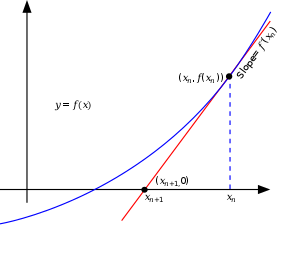
At the point $x=x_0$, The tangent line is given by the equation
And we solve the equation: $y=0$, i.e.: we find where does the tangent line cut the axis. This gives:
And this value is our next value of the estimate, which we shall call $x_1$. Of course, we repeat this argument over and over again, until the value does not change. Just a few iterations are needed. Then, we have a root of our function.
Our iteration can be written in this way:
This provides us with a rule to get $x_{n+1}$, i.e.: our next estimate, from $x_n$, i.e.: the previous one.
Let us see how it works in practice. Starting with $x=1$, we apply the rule and get:
> x=1;
> x-f(x)/df(x)
ans = 1.1675
And we get 1.1657 as our next estimate. We would like to work faster
than that, so we may just say:
> x=1;
> for n=1:20
> x=x-f(x)/df(x)
> endfor
If we ask now for $x$ (just type x in octave), you get 1.1447. If
you ask for $f(x)$, you get 1.224e-16 (in my machine, in yours it
may change), which is close enough to zero for me. You may want to
type format long in order to get many more digits and see that they
are all converged.
Exercises
-
Write a function that, when invoked, returns always the gaussian, $\exp(-x^2)$.
-
Consider a quadratic equation, $ax^2+bx+c=0$. Write a function that takes $a$, $b$ and $c$ as arguments and returns one of the solutions.
-
Write a
newtonfunction which takes an estimate and returns the value after (say) 20 iterations of Newton’s method. -
Solve the following equations with Newton’s method and check your results!
(a) $x^2=3$
(b) $\sin(x)=1/2-x$
(c) $\sin(\exp(x))=1/3$
- If you try to solve the equation $1-x^2=0$ and start out with $x_0=0$ you get into trouble. Why? How to get out of it?