Monte-Carlo techniques

Can randomness help us solve a problem? Yes, and in surprising ways. Of course, it can help us solve problems related to probability. For example:

I throw two dice. What are the chances that the sum of the two values is 8?

Imagine that we know no maths at all. We can still do an experiment: throw the dice one thousand times, and count how many times the sum of the two numbers is 7.

But the computer can do the experiment for us. It can throw random numbers which simulate the dice. Of course, there is nothing truly random in the procedure. Read this article in order to learn more about it.

We will adopt a pragmatic approach. Let us learn how to ask Octave to give us one random number:

> rand 
ans = 0.176546

If you get a different result, don’t worry: it’s random! We can also ask for a vector of random numbers:

> rand(1,10)

ans =  0.033603  0.844310  0.863146  0.336529  0.732133
       0.168386  0.251145  0.137676  0.839003  0.861589

It returns a matrix of size $1 \times 10$, full with random numbers chosen in $[0,1)$ (the right extreme, 1, can not show up). What if we want them to be random integers from 1 to 6? We can do the following:

[0,1) —(multiply by 6)—> [0,6) —(sum 1)—> [1,7) —(floor)—> {1,2,3,4,5,6}

What is that floor thing? It takes a number and returns the integer part, i.e.: $\lfloor x\rfloor$, the biggest integer which is lower than $x$. Putting it all together:

> floor(6*rand(1,10)+1)

ans =    5    5    6    5    1    4    2    1    2    6

OK, now the strategy seems more clear. Each time we do that, we get 10 runs of a die. Let us do it with two dice:

> R1 = floor(6*rand(1,10)+1);
> R2 = floor(6*rand(1,10)+1);
> Rtotal = R1+R2

Rtotal =

    6    3    7    9    6    5    7    7   11   10

Great. We see that the 7 comes more often than any other value. Is that just chance? We can plot the histogram of those data very easily:

> hist(Rtotal,11)

The “11” is because there are 11 different possible values: 2,3,…,12. We get

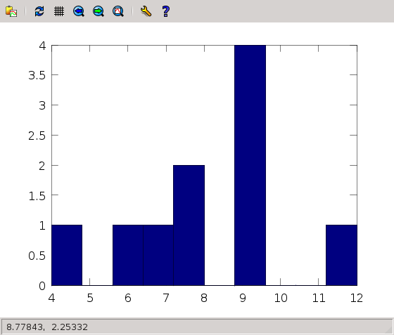
Hey, so many values… What if we improve that? Let’s repeat with 1000 values:

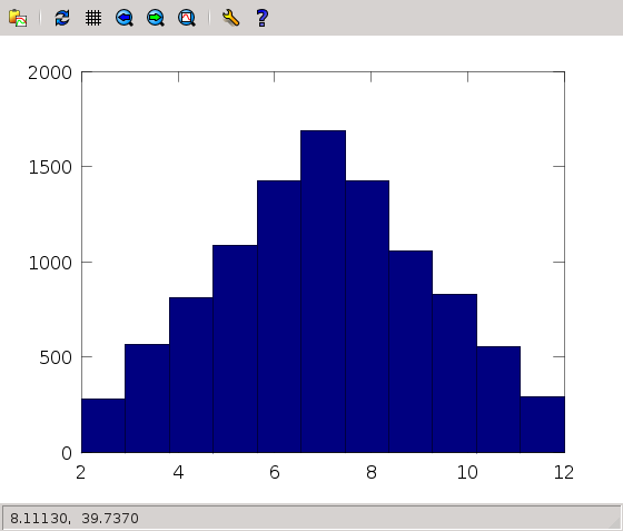
That’s a nice plot, for sure, but we would like to know how often does the 7 come up. No need to plot, just counting. Let N7 be the number of 7’s

> N7=0
> for n=1:10000
>     if (Rtotal(n)==7)
>        N7++;
>     endif
> endfor
> N7
ans = 1686

First: how does that program work? We run through all entries in vector Rtotal, with the for loop. Then, if the entry in question is 7 (if (Rtotal(n)==7)) we increment the count of N7. Here, we have introduced a new trick: N7++ is a shorthand for N7=N7+1, which I dislike a bit. A lot of new things in this short code.

Second: how to interpret the outcome? If there are 1686 sevens in 10000 runs, then we must say that the probability is close to 1686/10000 = 0.1686. Is that value right? OK, in this case probability theory gives us the exact number, it’s $1/6 \approx 0.1666$. Not bad.

Exercises

• What if we throw three dice? What is the value which gets the maximal probability? Get a similar histogram.

• I throw two dice 10000 times, but only annotate the maximum value of the two. Find the histogram, and get the probability of obtaining 6.

Finding the area of the circle

Monte Carlo methods is the name given to the technique for finding the answer to mathematical questions using random numbers in a computer. Let’s try to solve a very classical problem: to find the area of a circle with unit radius. Yes, I know, it’s $\pi$;. But we’ll do it in a very interesting way.

Let us get a 10 random points in the unit square $[0,1] \times [0,1]$, and plot them:

> x = rand(10,1);
> y = rand(10,1);
> scatter(x,y)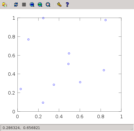

We use scatter instead of plot because we don’t want the points to be joined by a curve. Now, let us add a quarter of the unit circle:

> hold on  # this keeps the previous plot
> angle=0:0.1:pi/2;
> plot (cos(angle),sin(angle))

So, some of the points are inside the circle, some are outside. Let’s repeat it with 500 points:

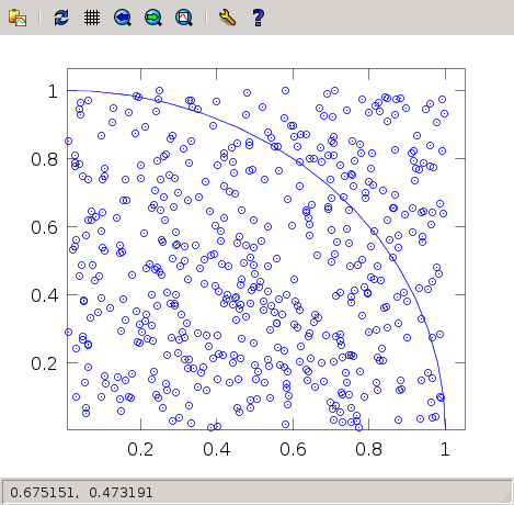
What is the probability of a given point being inside the curve? Well, it is proportional to the area of the circle quadrant divided by the area of the unit square (1). So, directly, the probability of finding a point inside, multiplied by 4, will give us the area of the circle!

If the point has coordinates $(x,y)$, how to know whether it is inside the circle? Easy: it is inside if its distance to the origin is smaller than 1: $x^2+y^2\leq 1$. We can ask Octave to check that for all points, and tell us the fraction.

Starting out the program again. Now, Ninside will count the number of points inside.

> Ninside=0; 
> x = rand(1,500); 
> y = rand(1,500); 
> for n = 1:500 
>   if (x(n)^2+y(n)^2 <= 1) 
>     Ninside++; 
>   endif 
> endfor 
> Ninside 
ans = 388 

(Caveat: you may get a different number, it’s random!)

How to read the result? Well, our estimate for the probability of finding a point inside the circle quadrant is given by

388/500 = 0.776

Now, multiply that number by 4, and we get 3.104. It seems like very far from $\pi$, but we can improve the result by launching more points…

Exercises

• Repeat the computation with $10^6$ points. What is your estimate now?

• Find the volume of a unit sphere using Monte Carlo.

• Find the area under a hump of the cosine function, using Monte Carlo.