Plotting functions and curves

Plotting mathematical objects is both useful and beautiful. Today we will just scratch the surface of the vast area of mathematical computer graphics, but we hope to give you a hint of what it looks like.

As our first task, we will try to plot a function. Imagine that you don’t know any maths, but you have a powerful calculator. How do you plot a function? You make up a table with a lot of points, and put all those points in a graph. OK, let us have a try. Let’s say we want to plot the $f(x)=\sin(x)$ function.

Remember how to generate all $x$ values from 0 to 10 at once? That’s right, you just do x=0:10;. Now, you want to compute the sine of all those values and put the numbers on another vector. So, you do: y=sin(x);. Next, you give Octave the command to plot the result:

> x=0:10;
> y=sin(x);
> plot(x,y)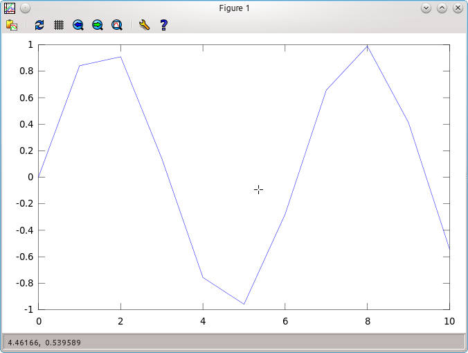

Of course, the command plot, takes two arguments: the vector of x values and the vector of y values, and plots them. But you can see that the plot is quite coarse and ugly. How to improve them? Right: give more points!!

> x=0:0.1:10;
> y=sin(x);
> plot(x,y)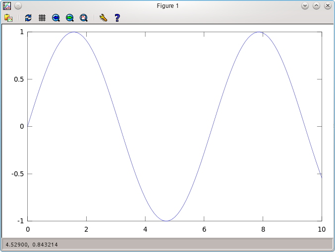

Of course, 0:0.1:10 means all numbers from 0 to 10, with steps of size 0.1, so we get 0, 0.1, 0.2, ... 1, 1.1, 1.2, ... 9.8, 9.9, 10. Thus, many more points. The plot is much smoother and nice.

You can also do several plots on the same screen very easily:

> x=0:0.1:10;
> y1=sin(x);
> y2=cos(x);
> plot(x,y1,x,y2);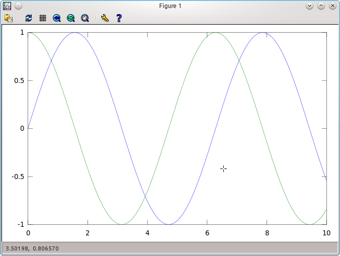

Remember that some functions require a dot in order to be properly evaluated for a vector. For example, x.^2, or 1./x. Thus, if we want to plot $f(x)=1/(1+x^2)$ in the range $x \in [-10,10]$, we have to do:

> x=-10:0.1:10;
> y=1./(1+x.^2);
> plot(x,y)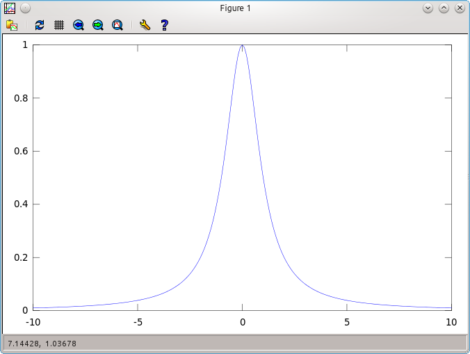

Polar Coordinates

The plot command is only useful to plot in cartesian coordinates. But, if we have a vector of $\theta$ values and another of $R$ values, we can convert them to cartesian coordinates with our usual expressions:

So, let us try an example. Let’s plot $R(\theta)=\theta $. We will give a wide range for $\theta$, in order to be sure that we catch it all.

> Theta=0:0.1:100;
> R=Theta;
> x=R.*cos(Theta);
> y=R.*sin(Theta);
> plot(x,y)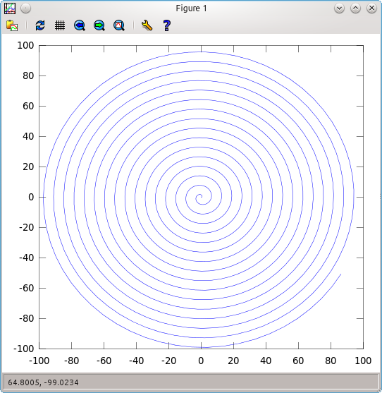

Now, for something more beautiful, we can try a polar rose, $R(\theta) = \cos(5\theta/12)$:

> Theta=0:0.1:100;
> R=cos((5/12)*Theta);
> x=R.*cos(Theta);
> y=R.*sin(Theta);
> plot(x,y)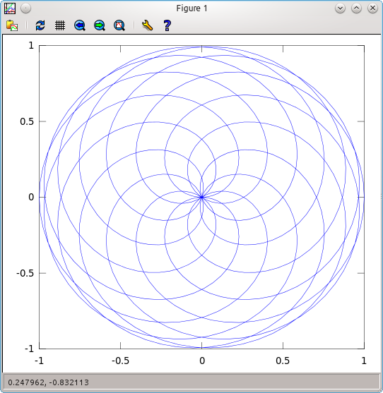

Exercises

• Plot the polynomial $y=1-x^2$ and the gaussian $y=\exp(-x^2)$.
• Draw an ellipse in polar coordinates, with semiaxes $a=2$ and $b=5$.
• A particle follows a trajectory given by the equations $x(t)=\sin(t)$, $y(t)=\sin(2t)$. Start getting a vector for your $t$ values, using t=0:0.1:20;, and use it to get an image of the trajectory.