Dynamical Systems

Let us discuss how to use Octave to solve systems of differential equations, and to plot phase diagrams of dynamical systems.

Summary of the basic theory

(Important note: this section is merely a reminder, not a substitute for a real discussion of dynamical systems. For details please refer to a serious book, such as Steven Strogatz’s Nonlinear Dynamics and Chaos.)

Let us consider a system of $n$ differential equations, such as

Given an initial condition, $(y_1(0),y_2(0),\cdots,y_n(0))$, and under some basic regularity conditions, there exists a single set of curves $(y_1(t),y_2(t),\cdots,y_n(t))$ satisfying the previous system of equations. For concreteness, we will usually work with $n=2$.

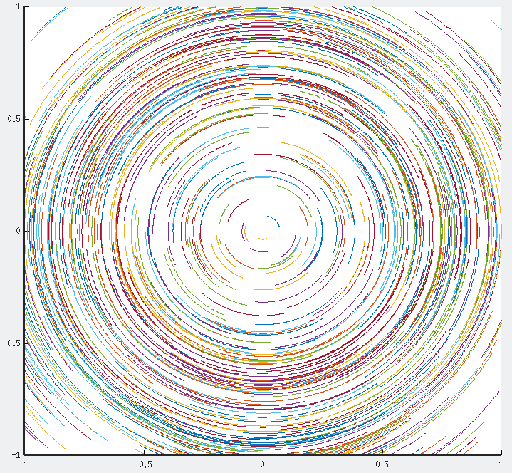
A very simple dynamical system is given by

whose integral curves are simply circumferences around the origin. Notice that differentiating again the first equation and substituting into the other we obtain

which is the differential equation for the harmonic oscillator. A more interesting example is provided by the van der Pol’s oscillator,

Numerically, these systems of equations can by solved using standard algorithms, such as Euler’s method or Runge-Kutta’s method. Luckily for us, Octave has those methods programmed.

Dynamical sytems in Octave

Let’s play a bit with Octave. We can define the differential equation using a function handle. For example, the harmonic oscillator is written as

> df = @(t,y) [y(2); -y(1)];

The @ symbol is shorthand for the function arguments: time $t$ and the values of $y$. Now, we make use of the ode45 function, which employs an algorithm which is equivalent to an order 4 Runge-Kutta. Function ode45 requires the following argument:

• Function handle.
• Values of t where we want the solution evaluated.
• Initial condition.

So, for example, we write

> [t,y] = ode45 (df, [0:0.01:1], [1,0]);

The syntax [t,y] on the left-hand-side means that the output should be placed on variables t and y. Notice that, as promised, the first argument is the function handle df. The second argument is the set of values of $t$ where we need the function defined, from 0 to 1 in steps of 0.01, so [0:0.01:1]. And the last, we provide the initial values at the first point, $y_1(0)=1$ and $y_2(0)=0$ in the form $[1,0]$.

Now, we have the final curve in $y$, which is a matrix, as we can readily check by printing it on the screen. In order to plot it, we do the following

> X=y(:,1);
> Y=y(:,2);
> plot(X,y)

But in order to visualize a full dynamical system we should be able to plot many such curves. We will write a short program that does precisely that:

• Chooses randomly $N=1000$ random initial points in a window, such as $[0,1]\times [0,1]$.

• Obtains the integral curves for a short time.

• Plots all the results together.

This is the final code:

> df = @(t,y) [y(2); -y(1)];
> hold on % For multiple plot
> pbaspect([1 1 1]) % To scale both axes equally
> xmin=-3; xmax=3; % Choosing the window of initial values
> ymin=-3; ymax=3;
> axis ([xmin xmax ymin ymax]) % To draw only in that window
> for n=1:500
>    x0=(xmax-xmin)*rand+xmin; y0=(ymax-ymin)*rand+ymin;
>    [t,y] = ode45 (df, [0:0.01:1], [x0, y0]);
>    X=y(:,1);
>    Y=y(:,2);
>    plot(X,Y)
>endfor

And the result should look as follows

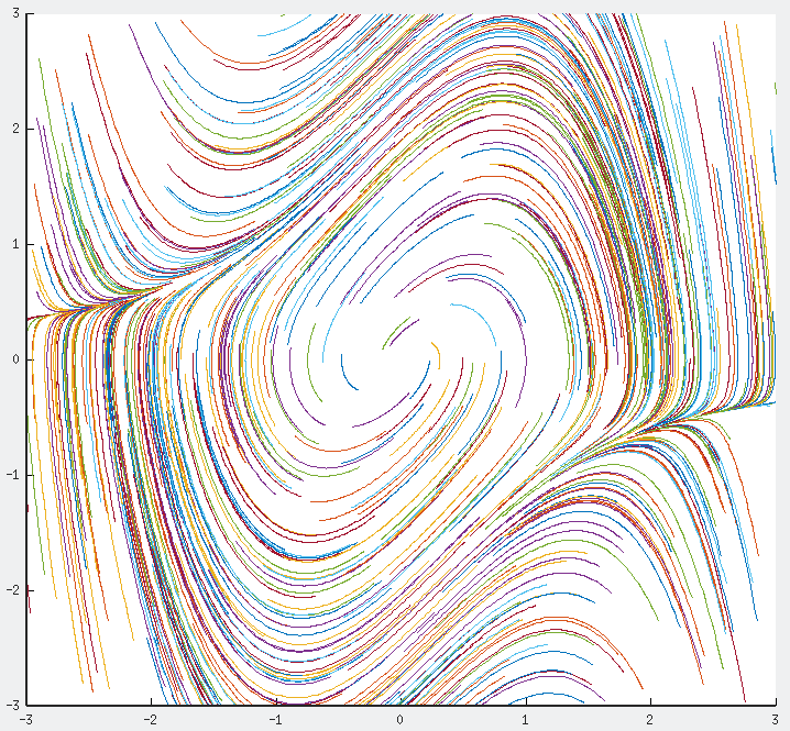
For van der Pol’s oscillator, use

> df = @(t,y) [y(2); (1 - y(1)^2) * y(2) - y(1)]; % Van der Pol's oscillator

in order to obtain

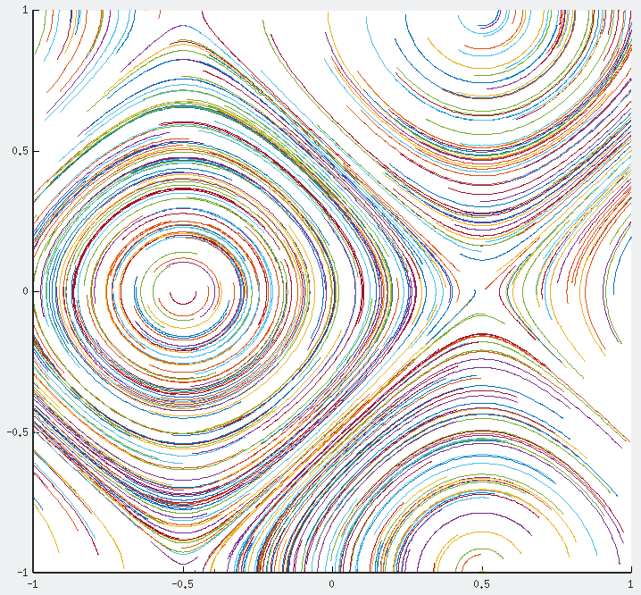
And you can try one more:

in the range $[-1,1]\times [-1,1]$ to obtain

It is convenient to use a full Octave script, such as

% script phase_diag.m
1;
pbaspect([1 1 1])
xmin=-1; xmax=1;
ymin=-1; ymax=1;

% df = @(t,y) [y(2); (1 - y(1)^2) * y(2) - y(1)];
% df = @(t,y) [y(2); -y(1)];
df = @(t,y) [sin(y(2)*pi); -cos(y(1)*pi)];

hold off
newplot
hold on
axis ([xmin xmax ymin ymax])

for n=1:500
  x0=(xmax-xmin)*rand+xmin; y0=(ymax-ymin)*rand+ymin;
  [t,y] = ode45 (df, [0:0.01:1], [x0, y0]);
  X=y(:,1);
  Y=y(:,2);
  plot(X,Y)
endfor

Thus, using these numerical techniques can help us understand the structure of the dynamical systems. For example, we can spot critical points and guess their nature. Of course, numerics is never a substitute for real analytical work, when it can be done. Thus, we can use Octave either to get some intuition about a new dynamical system, or to check what we have already found using analytical tools.