Differential Equations

This is most difficult part of the tutorial… So, please, pay a lot of attention and do all the exercises as you read.

The radioactive decay problem

Let’s start out with radioactive decay. Let us consider a certain radioactive substance that has two types of atoms: unstable and stable. The unstable atoms sometimes decay, emitting radiation, and becoming stable after that. It can be observed that the amount of radiation decreases with time. That’s because the number of unstable atoms decreses with time.

Let us model the radioactive decay in this way. Let $u(t)$ be the number of unstable atoms at time $t$. Let us consider a very very small time interval, from $t$ to $t+\Delta t$. The number of decaying atoms during that small interval should be proportional to the number of unstable atoms, and to the interval length:

where $K$ is just a proportionality constant. This is only true as a limit, when $\Delta t$ approaches zero. At time $t+\Delta t$ the number of unstable atoms will have decreased in that amount:

If we take the limit, $\Delta t \to 0$, we can read the time derivative of $u(t)$ from there:

That is a differential equation, i.e.: an equation for a function in which the value of the function and its derivatives are mixed up. How to solve it? There are two ways: (1) analytical, (2) numerical. We’ll do the analytical solution pretty fast, and then move on to the numerical computation, which is our point.

We’re being asked to write down a function such that, when you derivate it, you get something similar to itself, but multiplied by $-K$. I propose: $u(t) = A \exp(-Kt)$. And it is clear that any $A$ will do.

But what is $A$, anyway? OK, let us find the number of unstable atoms at the initial time $t=0$: $u(0) = A \exp(0) = A$, so now we know: $A$ is the initial value of the function, that should also be given to us.

A very important note: the same as with integrals, most differential equations do not have an analytical solution, so we have to recourse to numerical computation. But there is a difference: numerical integration is an easy task: it’s normally not worth to spend a lot of time integrating with pencil and paper when a computer can solve it for you in a couple of minutes. But numerical solution of differential equations, on the other hand, can be very challenging. So it is very worth to try to get as much analytical information about the solution as we can.

Numerical solution

First of all, let us formulate the problem a little bit more clearly. There are 1000 unstable atoms at a given moment in a sample with decay constant $K=1 s^{-1}$. Find the number of unstable atoms after one second.

OK, let us pretend that we don’t know about the analytical solution, and return to the previous equation:

Let us choose a small enough $\Delta t$, for example 0.1. Now we can proceed this way:

You can continue and, when you reach $t=1$, just read the value. Of course, as it is always the case, the smaller the $\Delta t$ the better the result! Can you figure out an Octave program to do it?

OK, let us start by defining the $\Delta t$

> dt = 0.1

We’ll store all the individual values for the $u(t)$ in a vector. How many of them shall we need? Not hard: $u(0)$, $u(0.1)$… $u(1)$. They’re 11. But we want it in general:

> N = 1/dt + 1

Next step, define the $K$:

> K=1

The idea now is to create a vector u such that u(1) corresponds to $u(0)$, u(2) corresponds to $u(\Delta t)$… until u(N) corresponds to $u(1)$. When we finish, we only have to print u(N) and we’re done.

So, we can do it the slow way:

> u(1) = 1000
> u(2) = u(1) - K * u(1) * dt
> u(3) = u(2) - K * u(2) * dt
...

But we can be more clever and use a loop:

> u(1)=1000;
> for i=1:N-1
>     u(i+1)=u(i)-K*u(i)*dt;
> endfor
> u(N)
ans = 348.68

Now just print u(N): 348.68.

• Is that value good or bad? In other terms: find the exact value and compare them. Hint: Give the command format long, so that numers are printed with twice the number of digits.

• Change the dt. Show in a table how u(N) approaches the exact value as dt decreases.

• Create a vector of times, t=0:dt:1 and plot the result for $u(t)$. Check with the exact solution, $u(t)=1000 \exp(-t)$. Do it for longer times, say $t=10$.

The harmonic oscillator

Let us consider a mass $m$ hanging from a spring, as in the pic:

And let us forget gravity, friction and everything else. We want to predict where is the mass going to be for any time $t$, so we’re asking for a function: $y(t)$. Let $y=0$ be the equilibrium position of the mass.

The only force acting on the particle is the spring tension, so Newton’s law reads:

and the minus sign is due to the fact that the tension is always opposite to the stretching. Given that $a(t)=y’‘(t)$, we have

And we have another differential equation, but this one is second order, because there appears a second derivative…

Let us reason in physical terms. Let us stretch the particle and leave it alone. Then, following the force, it comes to the equilibrium position… There, at the equilibrium position, the force is zero. But it does not stop!! It continues, because of the inertia, and oscillates, back and forth…

So, both the position and the velocity are relevant. Let $v(t)=y’(t)$, and $a(t)=y’‘(t)$. We are given the initial values of the position and velocity: $y(0)$ and $v(0)$.

Let us consider a small small time interval, $[t,t+\Delta t]$. If it is really small, the acceleration can be considered to be constant, equal to:

and then we just write down the equation for a motion with constant acceleration in that small time interval:

Of course, the velocity must be also updated:

That’s all! We’re asked now where is the particle at time $t=10$, if $k=m=1$, $y(0)=1$, $v(0)=0$.

Now, we try to put it all together in a program:

> dt = 0.1; # The value of Δt 
> tmax = 10; # The time we want to reach 
> k = 1;
> m = 1;
> N = tmax/dt + 1; # Number of time steps 
> y(1) = 1; # The initial position 
> v(1) = 0; # The initial velocity 
> a(1) = -(k/m)*y(1); # The initial acceleration 
> for i=1:N-1 
>     y(i+1) = y(i) + v(i)*dt + 0.5*a(i)*dt^2;
>     v(i+1) = v(i) + a(i)*dt;
>     a(i+1) = -(k/m)*y(i);
> endfor

Now you can just read y(N), you’ll get -1.0675.

Wait!! That value makes me think… I started the oscillator without initial velocity from an initial amplitude of $1$! How can I get values larger than that for the position???

Of course, the key is that the $\Delta t$ is too large. So, here comes the first problem:

• Show, in a table, how the previous value for $y(N)$ approaches its exact value as $\Delta t$ decreases. The exact solution is $y(t)=\cos(t)$. Check with it.

• Plot $y(t)$ and $\cos(t)$, together, for a small enough $\Delta t$. You should see something like this:

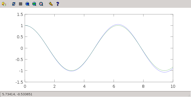
For an interesting plot, get $v$ versus $y$.

• (Extra) Are you able to add a damping term to the equation? Let the force be $F=-kx-\gamma v$. This is a way to model friction with a fluid medium, like air or water.